 Excel XLOOKUP Function Tutorial (with Pirates).
The Excel XLOOKUP Function Explained

What is XLOOKUP?
Very briefly, XLOOKUP is a versatile built-in Excel lookup function that can cross-reference data in two different columns vertically. Or, it can cross-reference data in two different rows horizontally. It then allows you to perform actions upon the data which has been "discovered" through the process of cross-referencing.
In this XLOOKUP Function tutorial we walk you through several fun examples of this incredibly useful Excel function in action, from the most basic three-part XLOOKUP to performing vertical and horizontal lookups with XLOOKUP, using [if_not_found], [match_mode] and [search_mode] arguments and also nesting XLOOKUP inside other functions including the =IF and =CONCAT functions to construct some more powerful formulas.
Difficulty: This XLOOKUP tutorial has an intermediate level of difficulty and is best-suited to those already confident using Microsoft Excel at a beginners level. It is also intended for anyone who is looking to make the transition from VLOOKUP to XLOOKUP.
You can download the Excel Workbook for this tutorial which has all of the data, formulas and working examples of XLOOKUP in there to use for reference in this tutorial.
Filename: "excel_xlookup_function_workbook.xlsx"
Size: 146KB
XLOOKUP LESSONS
- What's so good about XLOOKUP?
- What is the difference between Excel's XLOOKUP and VLOOKUP functions?
- What is the most basic syntax of the XLOOKUP function?
- Which Versions of Excel is the XLOOKUP Function Compatible with?
- Why is this Function Called XLOOKUP?
- Getting Started with Excel's XLOOKUP Function
- Excel XLOOKUP Function using the [if_not_found] Argument
- Retrieve Multiple Cells from an XLOOKUP Function
- Excel XLOOKUP Function nested in an IF Function
- A reminder that Excel's XLOOKUP Function can look both ways
- Using [match_mode] in an XLOOKUP Function
- Conditional XLOOKUP nested alongside IF within the CONCAT Function
- XLOOKUP Function with a Horizontal Lookup
- The XLOOKUP Function [search_mode] argument
- XLOOKUP Tutorial Conclusion
What's so good about XLOOKUP?
What makes XLOOKUP so great is its versatility. XLOOKUP can perform horizontal lookups like HLOOKUP and it can perform vertical lookups like VLOOKUP.
XLOOKUP not only does the job of two other older Excel functions (VLOOKUP and HLOOKUP), it also surpasses them both.
XLOOKUP Versus VLOOKUP
VLOOKUP can look from one column on the left to perform a vertical search on the content of another column to the right of it, but it can't look left. XLOOKUP can lookup the contents of columns in either direction.
Plus, the most basic VLOOKUP statement consists of four core parts where as XLOOKUP only needs three making it not only more powerful but also less complicated to master.
XLOOKUP Versus HLOOKUP
The most basic HLOOKUP statement consists of four core parts where as XLOOKUP only needs three making it not only more powerful but also less complicated to master.
What is the difference between Excel's XLOOKUP and VLOOKUP functions?
VLOOKUP
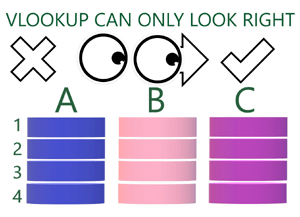
VLOOKUP can only look right (from a column on the left to a column on the right)
XLOOKUP
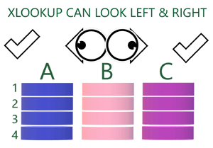
XLOOKUP can look both ways (from a column on the right to a column on the left, or from a column on the left to a column on the right).
And that's not all! XLOOKUP can also perform Horizontal lookups on rows, meaning that you can now look up and down as well; something which previously you needed to use HLOOKUP for.
So, if you already know something about VLOOKUP or HLOOKUP you're definitely going to want to learn to master XLOOKUP. Or, if you're new to Excel you can save yourself some time by learning just XLOOKUP rather than learning both VLOOKUP and HLOOKUP.
What is the most basic syntax of the XLOOKUP function?
You write out the syntax of a simple XLOOKUP function as follows:
=XLOOKUP("Jolly Seadog",A4:A11,B4:B11)
The basic XLOOKUP syntax consists of three comma-separated arguments.
- The first argument is the content of a cell from column A that we want to perform a lookup on ('Jolly Seadog'). This is known as the 'lookup_value'.
- The second argument is the cell range of our table in column A. This is known as the 'lookup_array' and it looks in Column A to find a match for this exact name.
- The third argument is the cell range of our table of data in column B that we want to use to look up our result. This is known as the 'return_array' and this takes the match from Column A (Jolly Seadog) and uses it to return the result from the same row in Column B (First Mate).
If you place your cursor into the formula editor you will see that Excel shows you the entire syntax structure of the function as follows:
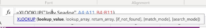
XLOOKUP (lookup_value, lookup_array, return_array, [if_not_found], [match_mode], [search_mode])
As you can see, XLOOKUP also has some additional optional arguments in its syntax: [if_not_found], [match_mode] and [search_mode].
We will provide some examples of these in action as we work through the lessons.
Back to topWhich Versions of Excel is the XLOOKUP Function Compatible with?
XLOOKUP was only released in 2020 and its not so long since only Office Insiders had access to it. As such it is only available in Excel versions Excel 365 and Excel 2021 for Windows and for Mac. It is also available on some Apple and Android mobile devices.
If you're using an earlier version of Excel then you can look at our VLOOKUP Function tutorial instead.
Why is this Function Called XLOOKUP?

It would be nice to think that the XLOOKUP function owes its name to treasure maps in which X marks the spot and where you're literally looking for X as part of a treasure hunt.
However, VLOOKUP is named for its ability to perform vertical lookups upon columns of data and HLOOKUP is named for its ability to perform horizontal lookups upon rows of data. As such, it seems highly likely that XLOOKUP is named so because the shape of the letter X reflects that XLOOKUP allows you to search multi-directionally (both vertically and horizontally).
Nonetheless the pirate analogy for XLOOKUP feels right, not least because the directional limitations of XLOOKUP's predecessor VLOOKUP make it seem like it has a patch over its left eye like a pirate. So we are going to run with a pirate theme in this article.
Getting Started with Excel's XLOOKUP Function
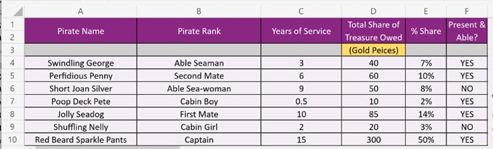
In this tutorial we use the scenario of a crew of pirates who have discovered a treasure chest and allocated each shipmate a portion of the treasure. We are going to use the XLOOKUP function to ensure that everyone who is entitled gets paid their rightful share.
We will start by using one XLOOKUP function to verify the identity of each crew member by rank and to catch any imposters who might be making false claims on the reward.
We will then use a second XLOOKUP function to determine which crew members should be paid now and who should be paid later before working through a variety of other ways to work with XLOOKUP.
Here is the Excel table with all of our data upon which we are going to perform our XLOOKUPs.
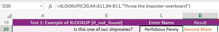
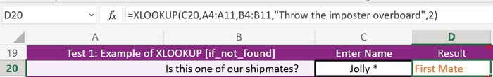
Excel XLOOKUP Function using the [if_not_found] Argument
=XLOOKUP(C20,A4:A11,B4:B11,"Throw the imposter overboard")
In this XLOOKUP we are going to test the value that is entered into cell C20, in order to look up the rank of the crew mate name entered.
You will notice that (unlike our basic XLOOKUP example which was made up of three comma-separated parts) this XLOOKUP is made up of four comma-separated parts. Also, rather than including the lookup_value for the sailor's name in the formula, we call the name from Cell C20, which allows a user to type a name into that cell and generate a result from our XLOOKUP.
This XLOOKUP takes the roster of crew members in COLUMN A and looks up their rank in COLUMN B. The lookup then makes use of the [if_not_found] statement to display text if the name that is entered in cell C20 is not found in COLUMN A.
So now when we enter the name of the crew member 'Perfidious Penny' into Cell C20 we get the following result which returns her rank:
But, if we enter into Cell C20 the name of a sailor that does not appear in our table we get a result as follows:
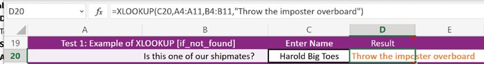
The name of the sailor 'Harold Big Toes' is not found in our Excel table so XLOOKUP can not return a rank for him and falls back on the [if_not_found] statement to provide us with an alternate course of action.
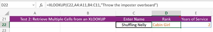
Back to topRetrieve Multiple Cells from an XLOOKUP Function
This XLOOKUP extends upon our previous example by adding an extra column to the return_array cell range which now extends from B4 to C11 and retrieves results from both the 'Rank' column and 'Years of Service' column. This allows us to perform an extra check to verify the identity of the crew member before giving them their payout.
=XLOOKUP(C22,A4:A11,B4:C11,"Throw the imposter overboard")
Excel XLOOKUP Function nested in an IF Function
In this example we use our XLOOKUP function to ensure that only serving members of the crew get paid and also that any crew member who isn't present and able has their share put aside for later.
We are going to nest our XLOOKUP within Excel's IF Function to add an extra layer of conditionality.
In the above two examples using XLOOKUP's [if_not_found] statement we could only do something when a certain condition was not met (e.g. the name of 'Harold Big Toes' did not appear in the table that we looked up).
By nesting XLOOKUP within an IF function we can now perform one action if our test is true and perform a different action if the result of our test is untrue.
Our formula with a nested XLOOKUP function looks as follows:
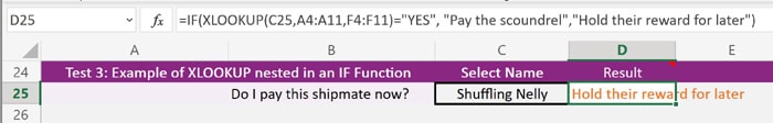
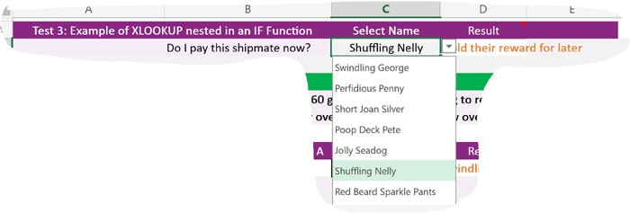
=IF(XLOOKUP(C23,A4:A11,F4:F11)="YES", "Pay the scoundrel","Hold their reward for later")
You will notice that the XLOOKUP function part of the formula looks pretty much the same as in previous examples, except that it is now no longer preceded by an equals sign.
Because the XLOOKUP function is nested, only the exterior function (IF) needs to have an equals sign.
The IF Function consists of three comma-separated parts, and our XLOOKUP makes up the first part of this which is the logical_test. In this part we run the XLOOKUP to match the name selected in cell C25 with a name in column A which then looks up Column F to check whether this sailor is 'Present and Able'.
Part one of the IF Function (using XLOOKUP):
XLOOKUP(C23,A4:A11,F4:F11)="YES",
Part two of the IF Function:
The second comma-separated part of the IF function tells Excel what information to display if the logical_test performed in the first part is true.
"Pay the scoundrel",
Part three of the IF Function:
The third comma separated part of the IF function tells Excel what information to display if the logical_test performed in the first part is untrue.
"Hold their reward for later"
As you can see, Excel's XLOOKUP function can suddenly become a lot more useful (and powerful) once you learn to combine it with or nest it within other Excel functions.
Note: Using Data Validation for Your XLOOKUP lookup_value
In this example of the XLOOKUP function we used a dropdown box for the data to use in the logical_test part of the function, so that users select the name from a list rather than entering it manually.
In order to do this for yourself, select the cell you want to add the dropdown box to. Then go to the Data tab and then select Data Validation. This will open the following dialog:
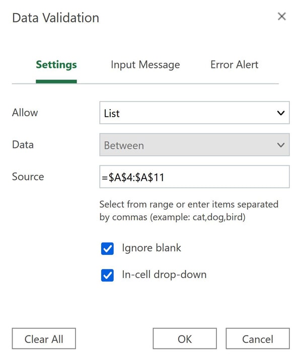
Choose 'List' from the options available in the 'Allow' dropdown and then put your cursor inside the 'Source' edit box and this will allow you to go back to your Sheet and select the range of cells you want to include in your dropdown.
Back to topA reminder that Excel's XLOOKUP Function can look both ways.
With this formula we are simply demonstrating that the XLOOKUP Function can do something that VLOOKUP can't. Excel's XLOOKUP Function can look both ways.
We are using this example of XLOOKUP to match the amount of gold peices owed to each sailor. So we use Column D for our lookup_array which contains the values for the treasure owed and we use Column A for our return_array which contains the names of the sailors.
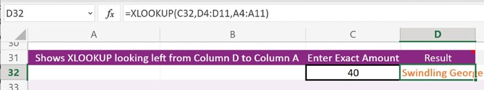
=XLOOKUP(C32,D4:D11,A4:A11)
In previous examples our XLOOKUPs have looked right from Column A to either Column B or Column F.
Here XLOOKUP uses Column D as its lookup_array which looks-up Column A (the return_array). XLOOKUP is looking from the right column to the left column. If we were to try to do this with VLOOKUP it would return an error, but here we have a perfectly well-constructed XLOOKUP function:
Using [match_mode] in an XLOOKUP Function.
Our previous XLOOKUP Function example has a flaw whereby if we don't enter an exact amount into Cell C32 it will return an error ('#N/A') because that amount does not exist in Column D of our table.
We can add an improvement to our formula by using XLOOKUP's [match_mode] argument.
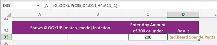
=XLOOKUP(C35,D4:D11,A4:A11,,1)
The first thing to take note of here is that we use two commas to bypass or stepover where the [if_not_found] argument would usually be declared. In this instance, we do not need the [if_not_found] argument, so we can step past it to get to the [match_mode] argument.
In this XLOOKUP you can enter any amount of treasure (equal to or less than the highest amount of treasure earnt: 300) and if an exact amount is not found XLOOKUP will use [match_mode] to find the pirate that earnt the closest amount searching upwards from the number you entered. Change the value from "1" to "-1" to find the sailor who earnt next less to this amount.
XLOOKUP's [match_mode] has other variables that you can take advantage of too.
- "0" will look for an exact match. This is the default setting and no different to not specifiying [match_mode] at all.
- "-1" If an exact match is not found then this will return the next smallest value.
- "1" If an exact match is not found then this will return the next highest value.
- "2" enables you to make use of wildcards. So, for instance, if we set [match_mode] to "2" in this example, we can then use wildcards in our lookup_value in Cell C35.
XLOOKUP [match_mode] with Wildcards.
If we go back to our earlier example in which we used [if_not_found] with our XLOOKUP function, we can now add [match_mode] to this to work with wildcards in our [lookup_value].
Our original XLOOKUP was written as follows:
=XLOOKUP(C20,A4:A11,B4:B11,"Throw the imposter overboard")
We are now going to extend this formula to set the [match_mode] to "2" for wildcards.
=XLOOKUP(C20,A4:A11,B4:B11,"Throw the imposter overboard",2)
This allows us to add wildcards to the searches that we input into Cell C20.
So, imagine that we want to find out which rank is held by Jolly Seadog, but we didn't know his last name. Here we could now use the wildcard asterick '*' after this sailor's first name as a wildcard to stand in for their surname as follows to return the answer of 'First Mate':
If you would like to learn more about using wildcards in XLOOKUP's [match_mode] you can refer to Microsoft's Excel support documentation for XLOOKUP.
Back to topConditional XLOOKUP nested alongside IF within the CONCAT Function
We have previously seen that we can nest an XLOOKUP within Excel's IF Function to add an extra layer of conditionality to a formula. Here we are going to take this one step further and nest both an IF Function and an XLOOKUP Function inside Excel's CONCAT Function.
Using the CONCAT function allows us to take the results from two other functions and join them together in our results:
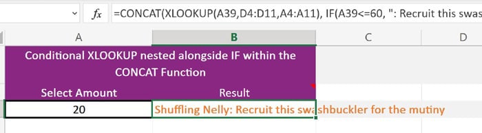
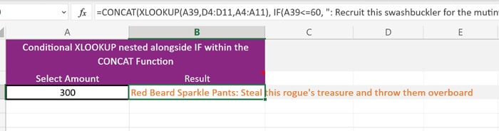
=CONCAT(XLOOKUP(C38,D4:D11,A4:A11), IF(C38<=60, ": Recruit this swashbuckler for the mutiny", ": Steal this rogue's treasure and throw them overboard"))
In this XLOOKUP example the formula will decide which action to take based upon the amount that you select. In this instance we want to know both what to do if the amount is less than or equal to 60 and also if the amount greater than 60. This is more than XLOOKUP's '[if_not_found]' can handle, so in order to grab hold of some more versatile conditionality we have nested our XLOOKUP along with an IF Function, both wrapped inside CONCAT.
Our XLOOKUP function returns the name of the sailor and IF returns the appropriate course of action to take.
The CONCAT function adds the IF result to the end of the XLOOKUP result in our output.
As with our example of XLOOKUP nested in IF, we have used Data Validation to create a dropdown list of amounts to select from in this formula.
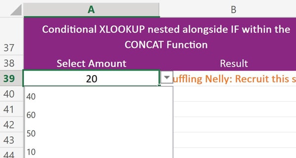
If we select a value from the dropdown of less than or equal to 60, the formula returns the result 'Recruit this swashbuckler':
However, if we select a value from the dropdown over 60 then when the IF Function checks to see whether the amount is less than or equal to 60, it returns an answer of false and displays the second string of text, 'Steal this rogue's treasure and throw them overboard'.
Other ways to Nest XLOOKUP
Note: There are also other ways to nest the XLOOKUP function. For instance, you could also nest two or more XLOOKUP functions within Excel's SUM function to calculate the total sum value of two or more output values. Try it for yourself.
You can even nest an XLOOKUP within another XLOOKUP Function. For instance, if you wanted to perform both horizontal and vertical lookups within just one formula.
XLOOKUP Function with a Horizontal Lookup
In this penultimate lesson we are going to look at a demonstration of Excel's XLOOKUP function peforming a horizontal lookup across rows, just like HLOOKUP.
For this last part of the XLOOKUP tutorial you will need to refer to the second Sheet in the Workbook that we have provided for download called 'Rum Ration (Horizontal XLOOKUP)'.

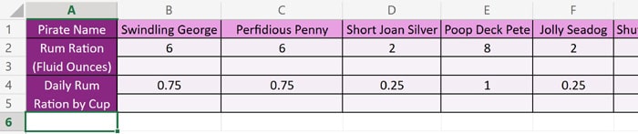
In our table we have recorded the unit amount of each sailor's alloted daily rum ration in fluid ounces in Row 2. Then in Row 4 we have used Excel's CONVERT function to convert these units into a standard cup size.
Our Horizontal XLOOKUP appears as follows:
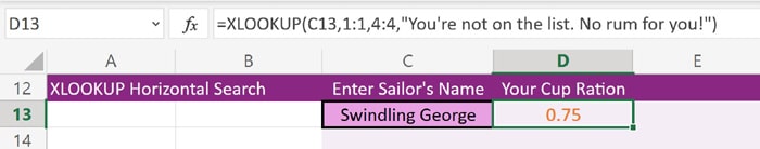
=XLOOKUP(C13,1:1,4:4,"You're not on the list. No rum for you!")
You can see here that both our lookup_array and return_array handle cell ranges slightly differently to the previous examples that we have encountered. For instance, the lookup_array looks from everything in Row 1 to everything in Row 1, with no reference to columns whatsoever. And the same goes for the return_array which looks from Row 4 to Row 4.
The formula will also work just fine if we use exact cell references for our cell ranges (as we have done previously), but this is a bit more longwinded:
=XLOOKUP(C13,B1:I1,B4:I4,"You're not on the list. No rum for you!")
This XLOOKUP will return exactly the same results as the one in which we only specify rows. It's just a longer way of going about it and since we are working horizontally by rows here it feels much more logical to define our cell ranges by just rows rather than by rows and columns.
Our XLOOKUP will look horizontally across the rows to assign the right cup ration to the right sailor.
Back to top
The XLOOKUP Function [search_mode] argument
In this final lesson covering the Excel LOOKUP function we are going to look at the sixth and final argument in XLOOKUP's syntax, the [search_mode] argument.
This is the argument that we might want to consider using in our XLOOKUP functions in instances where we have multiple cells which have the same values.
As we can see in our Rum Ration table, for instance, both Swindling George and Perfidious Penny are entitled to 6 fluid ounces of rum per day, and both Short Joan Silver and Jolly Seadog are entitled to 2 fluid ounces of rum per day.
So, if we wanted to lookup a crew member's name by their fluid ounce rum ration then it might be helpful to be able to set the direction of the lookup.
The XLOOKUP [search_mode] argument has a four different operators available to it.
- -1 Searches from the last item in the row or column through to the first item.
- 1 Searches from the first item in the row or column through to the last item.
- -2 To use this search you need to have your data sorted in descending order. Performs a binary search from the last item to the first.
- 2 To use this search you need to have your data sorted in ascending order. Performs a binary search from the first item to the last.
In this example we use search_mode to search ascending with the 1 operator.
=XLOOKUP(C16,2:2,1:1,"There's no ration of that volume",0,1)
Now when we enter a value of "2" into Cell C16 this returns the first match in Row 2 telling us that it is Short Joan Silver who entitled to this amount of fluid ounces of rum per day.
![XLOOKUP Function [search_mode] search ascending](ms_images/excel_xlookup_function/xlookup_function_search_mode_search_ascending.jpg)
If we change the [search_mode] value in our formula to minus 1, then Excel will start searching from the end of the row back to the beginning (search descending). This time the first match it encounters for the value of "2" fluid ounces is the sailor called Jolly Seadog.
=XLOOKUP(C16,2:2,1:1,"There's no ration of that volume",0,-1)
![XLOOKUP Function [search_mode] search descending](ms_images/excel_xlookup_function/xlookup_function_search_mode_search_descending.jpg)
Excel XLOOKUP Function Conclusion
As we have seen, Excel's XLOOKUP function is both versatile and powerful and can do an awful lot of work when it comes to manipulating data in your spreadsheets. Spend some time improving your knowledge of XLOOKUP and you will quickly get much more control over your spreadsheet data.
If you enjoyed this tutorial you might also like:
- 17 Excel Functions for Absolute Beginners
- DateDif() the Hidden Excel Function that You Should Know About
- The Best Places to Teach Yourself the Excel LAMBDA Function
- How do I translate Excel Functions into other Languages?
- Excel Sunburst Charts: Three Part Tutorial
- Create a Simple Excel VLOOKUP in Under 2 mins
- Concise Guide to Excel Shortcut Keys
- The Excel CONVERT Function Conversion Toolkit
- How Long Does it Take to Learn Excel?
We really ❤ helping organisations to master Microsoft Excel.
Our only question is: Will it be yours?
We come to you: Our regional Microsoft Excel trainers cover most locations of mainland UK for on-site visits including the English regions of the North West, North East, Yorkshire and the Humber, Greater London, the East of England, West Midlands, East Midlands, and also some parts of the South West of England (including Wiltshire, Bristol area and Gloucestershire) and South East of England (including Buckinghamshire, Oxfordshire, Berkshire, Hampshire and Surrey). Virtual classroom courses are available from anywhere via live video conferencing.

Our Excel Trainers are:
Inspirational subject experts with a wealth of experience, proven track records and excellent feedback.
Our Closed Excel Courses are:
Flexible instructor-led courses catering to YOUR specific learning needs and training requirements.
Education is Our Passion:
Over 35,000 students trained across almost every industry, sector and background.
Back to top
 Excel Training Reviews
An excellent, clear and patient tutor who guided me through the course seamlessly.
M Menzies (Online Excel training 365 (virtual classroom))
Can I just pass on my thanks to your team for the training you provided in York. I've had lots of positive feedback from the staff involved.
J Whiley, NHS York and Selby (Excel training York)
Really useful. Really knowledgeable trainer.
A Ward, Aeromet (Advanced Excel Training Worcester)
The trainer explained everything really well. I found the course easy to follow.
V Broxham, Baywa-re Operational Services (Intermediate Excel training Milton Keynes)
Happy with everything.
M Aston, Bierce Surveying Ltd (Advanced Excel Training Aylesbury Buckinghamshire)
We have had a few people over the years but the way the trainer picked up our business and requirements so quickly – all I can is you have a diamond there.
S Jenkins, Concorde Glass (Intermediate Excel Training Grimsby)
We all thoroughly enjoyed the course, we learned a great deal and thought Sara was a brilliant trainer, very patient with a fantastic way of teaching us, so thank you for that.
C Waldock, Darlington Borough Council (Intermediate Excel training Darlington, County Durham)
☆ ☆ ☆ ☆ ☆ Five Star Review
We had some really great feedback from the last two training sessions,
on the quality of the content as well as the delivery from the trainer.
Excel Training London
The content covered the exact content required after the beginners course. The information will allow me to improve the spreadsheets currently in use.
L Powell, Dudley Building Society (Intermediate Excel Training Dudley)
Great course!
V Franklin, E-Leather (Excel Beginners Training Peterborough)
The training approach and style was great. Incredibly informative and supportive.
L Shier, One YMCA (Introduction to Excel Training Watford, Hertfordshire)
Great teacher!
J Smith, Fisher German (Intermediate Excel Training Canterbury, Kent)
Its an excellent course. I was impressed by the discovery of so many tools that will facilitate our working life. The trainer is excellent, everything was perfect.
S Green, HW Martin (Beginners Excel Training Cambridgeshire)
Very happy to learn so much.
O Chawishly, LM Information Delivery (Intermediate Excel Training Oxfordshire)
Covered all objectives. Wish We'd had two days.
B Hough, Homebase (VBA for Excel Training Milton Keynes)
The course was excellent, covering more in a single day of training than I anticipated would be possible with a high degree of clarity.
Unsigned, New Economy, (VBA for Excel Training Manchester)
Very informative, easy to follow. Trainer was clear with his explanations
S Nottingham, Denney O'Hara (Microsoft Excel training Leeds, West Yorkshire)
Excellent day!
L McLachlan, Grange School (Excel training Rochdale, Greater Manchester)
Brilliant Training, went at the right speed [and] was made relevant to work
Kathryn Strong, Tennants Distribution (Excel training Manchester)
Fantastic course, not too much information overload. Explained simple. Exactly what I needed. Many thanks.
K Stobbs, Depuy Spine - A Jonson and Jonson Company (Introductory Excel training Leeds, West Yorkshire)
The flexibility of the course was ideal.
S Walsh, Progress Rail (Advanced Excel training Edinburgh, Midlothian)
The guys who came to the course this week were very impressed with the whole set up and are now eager to attend the next level up.
E Dixon, Connaught PLC (Beginners Excel training Leeds, West Yorkshire)
The course has improved my knowledge of Microsoft Excel and was a good pace so easily understandable. Gerry was very patient and helped each of us where we needed it.
L Muir, Filtronic Broadband (Microsoft Excel training Newcastle Upon Tyne)
Although a total beginner on Excel, I found the course to be extremely helpful.
S Antonie, Filtronic (Excel training Shipley)
Made what I thought was going to be completely foreign to me easy to understand. I can actually see where I can use Excel in my day job now. Max was very good and took the time to make sure we understood. [...] Nothing could be improved.
C Elsmore, Elmwood Design (Excel training Leeds, West Yorkshire)
Very Useful.
J Collins, Cooper Research Technology Ltd (Advanced MS Excel Training Ripley, Derbyshire)
Enjoyable and informative.
N. Bell, Cosalt PLC (Excel advanced training Grimsby, Lincolnshire)
The training session went very well and I have had a lot of good feedback from the participants.
P Ogden, InterfaceFLOR (Microsoft Excel Training Halifax West Yorkshire)
Course exceeded expectations.
K. Richards, Ashfield Homes (Microsoft Excel Training Sutton-in-Ashfield, Nottinghamshire)
The day was very well constructed and presented.
D. Coulthand, Crossgates Shopping Centre, Leeds (Intermediate Microsoft Excel Training Leeds, West Yorkshire)
Training very clear. Never felt rushed or pressured to complete tasks. Each item explained and demonstrated very well. Easy to follow
S. Hope, Lear Corporation (Advanced Microsoft Excel Training Coventry, West Midlands)
Good course, good information, good trainer and at a nice tempo
A. Webster, BE Aerospace (Advanced Microsoft Excel Training Hinckley, Leicestershire)
Excellent, the best Excel course I have ever been on. Trainer gave time and patience to us all.
D. Gill, Persimmon Homes (Beginners Microsoft Excel Training Malmesbury, Wiltshire)
A very robust day's training.
T. Camp, Ideal Shopping (Beginners Microsoft Excel Training Peterborough, Cambridgeshire)
The course in Edinburgh was incredible
C. Rowley (Beginners Microsoft Excel Training Edinburgh, Midlothian)
☆ ☆ ☆ ☆ ☆ Five Star Review
Thank You. We got very good feedback from all who
attended the beginners course last week.
Virtual Classroom Excel Training Glasgow
MS Excel Course Levels:
- Beginners Excel
- - introductory topics for working with Excel spreadsheets
- Intermediate Excel
- - conditional formatting, VLOOKUP, IF, apply formulas across worksheets, database features, security and conditional formatting etc.
- Advanced Excel
- - What-If Analysis, PivotTables, PivotCharts, Goal Seek, Sparklines, protecting workbooks, formula auditing etc.
- Masterclass Excel
- - 'zero to hero' three-day intensive Excel course
- Excel for VBA beginners
- - one or two day introduction to programming with VBA
- Excel Power Query course
- - Introduction to using Excel Power Query along with Pivot Tables, Power Pivot and Power Pivot Measures
- Copilot Integration with Microsoft Excel for Power Users course
- - Enterprise Microsoft Excel course to accelerate data analysis, automation and reporting using Copilot's native Excel integrations
To book a training course simply call 0844 493 3699, or email info@foursquaretraining.co.uk